Approach for Approximating Arbitrary Curves by NURBS

Ling Huang Jianfeng Zhen Xinxiong Zhu

（School of Mechanical Engineering & Automation,

Beijing University of Aeronautics & Astronautics, Beijing, 100083）

Abstract: All curves in the CAD/CAM system should be represented by NURBS. This paper presents an algorithm for approximating arbitrary curve by NURBS curve meeting the given tolerance with least number of data. It is the basis of representing offset curve(s) and surface/surface intersection curves in NURBS form and has been applied in the commercial CAD/CAE/CAM software system – CAXA-ME.

1. Introduction

NURBS have become the de facto standard for the representation, design and data exchange of geometric information processed by computers. All the curves in our CAD/CAM system should be represented by NURBS. For all elementary analytic curves，such as line, arc and conics, can be represented by NURBS precisely. But a number of advanced analytic and geometric curves widely used in free-form modeling, can’t be represented by NURBS precisely, for example:

l Surface/surface intersection curves ( Fig.1.a ).

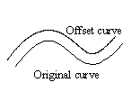
l Offset curves ( Fig.1.b ).

l

Implicit curves or curves represented by formulas, for example( Fig.1.c ):

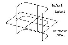
(a) Intersection curve (b) offset curve (c) formula represented curve

Fig.1. Curves need to be approximated by NURBS

Those curves can only be approximated by NURBS within a given tolerance.

This memorandum introduces a new method for approximating arbitrary curves called original curves by NURBS curves applying the techniques of curve fitting and error estimation. Given an arbitrary original curve by parametric representation (for example, offset curve) or by geometric equations (for example, surface/surface intersection curve), the goal of the algorithm is to construct a NURBS curve approximating the original curve with least numbers of segments in terms of the maximum deviation no more than the given tolerance. All positions and derivatives on the original curve can be calculated properly.

2. Strategy

2.1 Procedure

The procedure of approximating an arbitrary curve by a NURBS curve is as follows:

l Step1: Calculate the key points on original curve and divide it into many monotonic intervals.

l Step2: Construct a NURBS curve fitting the sample points (including key points) and get a candidate approximation curve.

l Step3: Estimate the deviation between the original curve and the candidate NURBS curve in every interval and check if the deviation is less than the given tolerance E.

l Step4: If all the deviations are less than tolerance E, the candidate NURBS is accepted. Otherwise, go to step5.

l Step5: Add new data point(s) into the sample points array at interval(s) where the deviation exceeds the given tolerance E. Go to step 2.

2.2 Calculations of Key Points

See Fig.2 and Fig.3, The key points on a curve, such as cusps, inflections and extremes, subdivide the curve into many monotonic intervals. We consider that the key points can reflect the main shape of the curve. It can be seen that the curve only interpolating the key points is almost the same as the original one. So the key points on a curve are important and helpful to the approximation procedure.

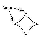
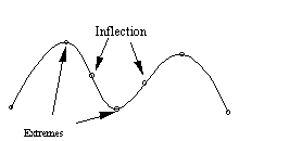
Fig.2. Key points on curve

Many achievements can be used to calculate the key points on curves. [Stone’89] analyzed the key points on parametric cubic curves by expressing the curve as a linear combination of control points and transforming it to the “canonical curve”. [Manocha’92] presented an algorithm to compute the proper parameterization of a curve and determined the cusps by the vanishing of the first derivative vector. [Manocha’92] also used the regular parameterizations to analyzed the inflection points.

Applying the algorithms presented by those authors, we calculate all the cusps and inflection points on the original curve which are denoted as points and unit tangent vectors at . These points serve as the point array for constructing the initial candidate NURBS curve.

2.3 Curve Construction

We first locally interpolate points by cubic Bezier segments and then compose all the Bezier segments to a candidate NURBS curve by selecting a suitable knot vector.

Given points and unit tangent vectors at , we can construct a number of cubic Bezier curve segments, , so that and are the endpoints of . Neighboring segments are joined together with continuity. Let denotes the control points of the Bezier segments which interpolate points of and and tangent vectors and , . Thus , , and and are unknowns. The Bezier segments can be represented as follows:

, ( 1 )

It is possible to construct a cubic Bezier curve satisfying the following constraint:

( 2 )

where , and are the derivatives of the cubic Bezier curve at parameters 0, and 1, respectively.

According to the properties of the derivatives at the end points of a cubic Bezier curve, Equation ( 2 ) implies that

( 3 )

( 4 )

where , are the first derivatives of the cubic Bernstein basis function. Combining Equations ( 2 ), ( 3 ) and ( 4 )，we can get two real solutions for . Substituting the positive solution into Equation ( 3 ) yields the desired two inner control points and . Every segment of can be generated by applying this algorithm and the neighboring segments are joined together with continuity. The Bezier segments can be composed to a NURBS curve by selecting a suitable knot vector. Applying the curve fitting algorithm described, we can get a candidate NURBS curve based on the sample points, consisting of key points and the point(s) added in interval(s) where the deviation is greater than the given tolerance E.

2.4 Error Estimation

The deviation between the candidate curve and the original one should be estimated. All the points interpolated by the NURBS curve are calculated from the original curve. Obviously, the candidate NURBS curve goes through those points precisely. So we should only estimate the deviation in the corresponding interval(s).

As shown in Fig.3, the dashed curve is the one interpolating key points and the real curve original one. Apparently, there is a maximum deviation between the approximated and the original curves in an interval. For convenience, we can consider that the maximum deviation in every interval is located at the point where the parameter value is the average of those corresponding to two adjacent interpolating points, such as the point M in the interval between points A and B on the original curve as shown in Fig.4.

Then, apply Equation ( 4 ), project point M to candidate curve and get point . is the distance from point M to the candidate curve and can be considered the maximum deviation in interval AB. The maximum deviation of all intervals can be calculated by:

( 5 )

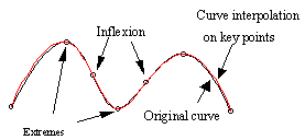
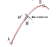
Fig.3. Curve interpolating key points Fig.4. Max deviation between two curves

2.5 Adding New Data Points

If the maximum deviation calculated by Equation ( 5 ) is less then the given tolerance, the procedure stops and the candidate NURBS curve is the right one. If the deviation in some interval(s) exceed(s) the given tolerance, the interval(s) should be subdivided. For example, if is less than the given tolerance, the candidate curve in interval AB meets the tolerance requirement; otherwise, we should subdivided interval AB to AM and MB by adding a point M to the initial point array that should be interpolated again. Estimate all the deviations interval by interval, add point(s) in interval(s) where the deviation does not reach the tolerance and generate a new NURBS curve. Repeating the procedure, we can get the candidate NURBS curves with less and less deviation. The procedure goes repeatedly until a satisfied curve is obtained.

3. Samples

We have applied the algorithm to the NURBS representations of surface/surface intersection curve, offset curve and formula represented curve as show in Fig.5, Fig.6 and Fig.7 respectively. This algorithm has been incorporated into our commercial CAD/CAE/CAM software system —CAXA-ME.

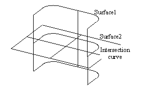
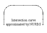
Fig.5. Approximation of Surface/surface intersection curve

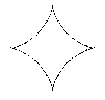
(a) The equation of the original curve (b) The curve approximated by NURBS

Fig.6. Approximation of formula represented curve

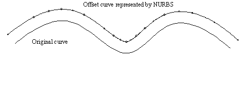
Fig.7. Approximation of offset curve

References

[1] Piegl,L. and Tiller,W., The NURBS Book, Springer, 1995.

[2] Stone,M.C. and DeRose,T.D., A Geometric Characterization of Parametric cubic Curves, ACM Transaction on Graphics, Vol.8, No.3, 1989, 147-163.

[3] Manocha,D. and Canny,J.F., Detecting Cusps and Inflection Points in Curves, Computer Aided Geometric Design, 9(1992),1-24.